This is the multi-page printable view of this section. Click here to print.
Documentation
1 - Getting Started
Hardware Installation
If you intend to power the HALPI computer via the NMEA 2000 network, the device is ready to use as-is! Connect the HALPI computer to the NMEA 2000 network using a Micro-C drop cable and a T-connector. To minimize voltage drop over the network backbone, it is recommended to place the HALPI computer close to the power feed.
If you intend to power HALPI using a dedicated power connector, you need to open the enclosure and replace the green NMEA 2000 power connector with the dedicated power connector. See the photo below. In this case, you need to solder a power cable to the provided SP13 cable plug. The maximum wire size for the connector is 2 mm² or 14 AWG.
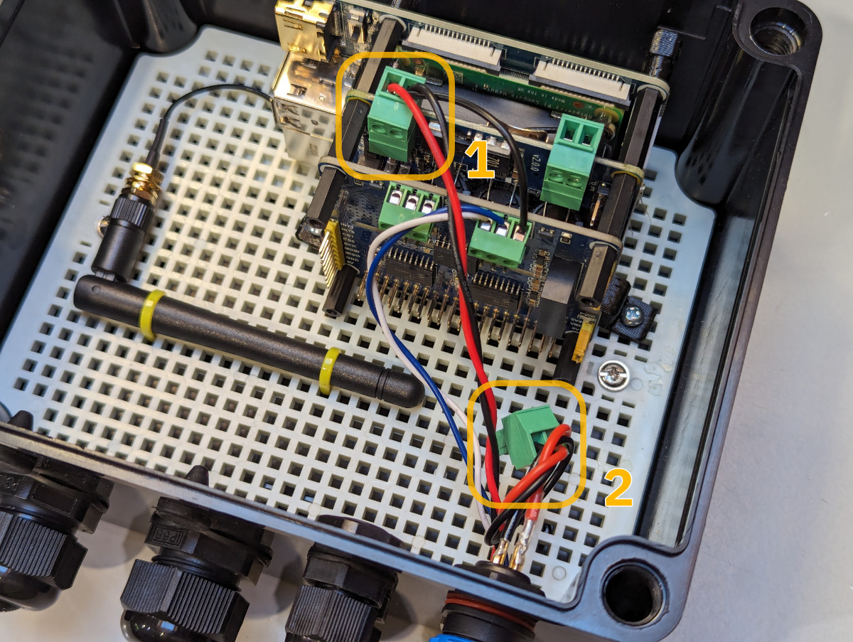
To power HALPI using a dedicated power connector, replace the green plug #1 with the plug #2.
Despite being waterproof, the enclosure should be protected from the elements. HALPI computers can be mounted in any orientation. If mounted on a wall, the enclosure should be mounted with the cable glands facing downwards or to the side to minimize the possibility of water ingress. Velcro tape is an excellent option for wall-mounting since it is relatively secure and allows for easy removal of the computer. The HALPI-M enclosure also allows for screw mounting using the 4 mm screw holes under the plastic lid screws. If a HALPI-S is to be screw-mounted, mounting tabs need to be devised and attached to the enclosure.
Initial Configuration
HALPI comes pre-installed with OpenPlotter 4 Headless edition. It can be used either with or without a display, keyboard, and mouse.
If you have display connected, follow the OpenPlotter 4 documentation to configure the system.
On a headless system, you will first need to connect to the WiFi Access Point created by the HALPI computer. Then, you can access the HALPI computer using VNC (or SSH) and carry on with the initial setup following the OpenPlotter 4 documentation. To use VNC, download VNC Viewer. VNC provides a remote desktop interface to access the HALPI desktop interface.
Important steps are to change the default password, the WiFi Access Point password, and to configure WiFi client settings if needed.
Configuring Signal K
Signal K is a modern and open-source universal marine data exchange format and server that can be used to connect various navigation software and hardware.
OpenPlotter 4 comes pre-installed with Signal K.
Basic interfaces such as NMEA 2000 and GPS, if any, are pre-configured, but you may need to adjust the settings to match your specific setup.
Access the Signal K web interface by navigating to http://openplotter.local:3000 in your web browser.
You can do that using your computer web browser or even a smartphone or tablet – it doesn’t have to be over the VNC Viewer.
Instructions for configuring Signal K can be found in the Signal K documentation.
2 - Hardware Description
HALPI-CM4 Hardware Description
The HALPI computers are based on the following component listed below. The list items link to the respective product documentation.
- Raspberry Pi Compute Module 4 with 4 or 8 GB of RAM, WiFi and no eMMC
- Waveshare CM4-IO-BASE-A Base Board, see also Wiki
- KingSpec M.2 NVMe SSD drive
- SH-RPi v2 Power Management HAT
- Waveshare CM4 3007 Cooling Fan
- Waveshare 2-Channel Isolated CAN HAT for NMEA 2000 connectivity, see also Wiki
- NMEA 2000 Pigtail Connector
- External WiFi antenna (mounted inside the enclosure)
Additionally, several optional accessories can be added to the HALPI-M:
- Waveshare 2-Channel Isolated RS485 HAT for NMEA 0183 connectivity, see also Wiki
- Waveshare MAX-M8Q GNSS HAT for GPS reception, see also Wiki
The HALPI-S does not have space for additional HATs.
3 - Software
Introduction
HALPI is a general-purpose computer that comes preinstalled with OpenPlotter 4, a custom distribution of Raspberry Pi OS with a number of pre-installed applications and services. HALPI’s OpenPlotter installation is slightly customized to support the hardware and software features of the HALPI computer.
Documentation for each software component is provided by their respective projects:
- Raspberry Pi OS: Raspberry Pi OS Documentation
- OpenPlotter: OpenPlotter Documentation
- Signal K: Signal K Documentation
- AvNav: AvNav Documentation
- OpenCPN: OpenCPN Documentation
Hat Labs provides some additional documentation relevant to common use cases of HALPI computers.
Software Updates
In normal conditions, incremental updates with Raspberry Pi OS and OpenPlotter are provided through the package manager and OpenPlotter facilities. However, if you need to reinstall the system, you can download OpenPlotter-HALPI images from the OpenPlotter-HALPI releases page.
Reinstalling the system will erase all data on the computer, so make sure to back up any important data before proceeding.
To install the image, you need to remove the SSD drive from the HALPI computer and connect it to another computer with an M.2 USB adapter. These adapters are available from various online retailers. The image can then be written to the SSD drive using Raspberry Pi Imager. Once done, unplug the USB cable, remove the drive from the adapter and reinsert it to the HALPI computer.
Data Logging and Visualization with InfluxDB and Grafana
A particularly powerful use case for HALPI computers is data logging and visualization. Signal K, together with the InfluxDB time-series database, can be used to log data from the NMEA 2000 network and other sources. Grafana, a popular analytics and visualization platform, can then be used to create dashboards and reports based on the logged data.
The SSD storage capacity of HALPI computers is sufficient for storing years of data. However, since we prefer to minimize unintended disk use, we do not enable data logging by default. Follow the instructions below to enable data logging and visualization.
InfluxDB Installation
InfluxDB v2 can be installed using the OpenPlotter desktop tools.
If you don’t have a display connected, use VNC Viewer to connect to the HALPI computer and open the OpenPlotter desktop.
Go to the top-left Raspberry menu -> OpenPlotter -> Dashboards:
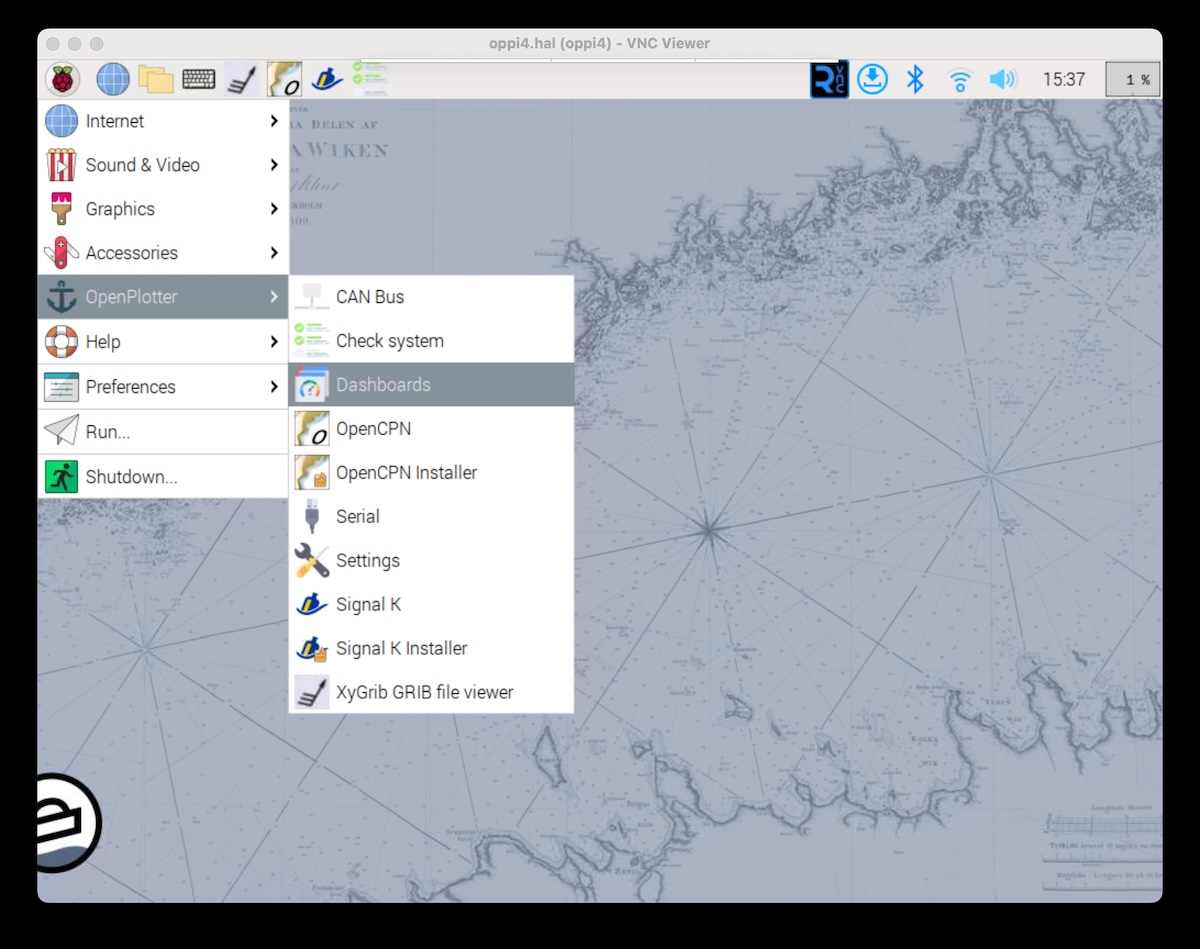
Open the Dashboards app.
Install InfluxDB OSS 2.x and Grafana.
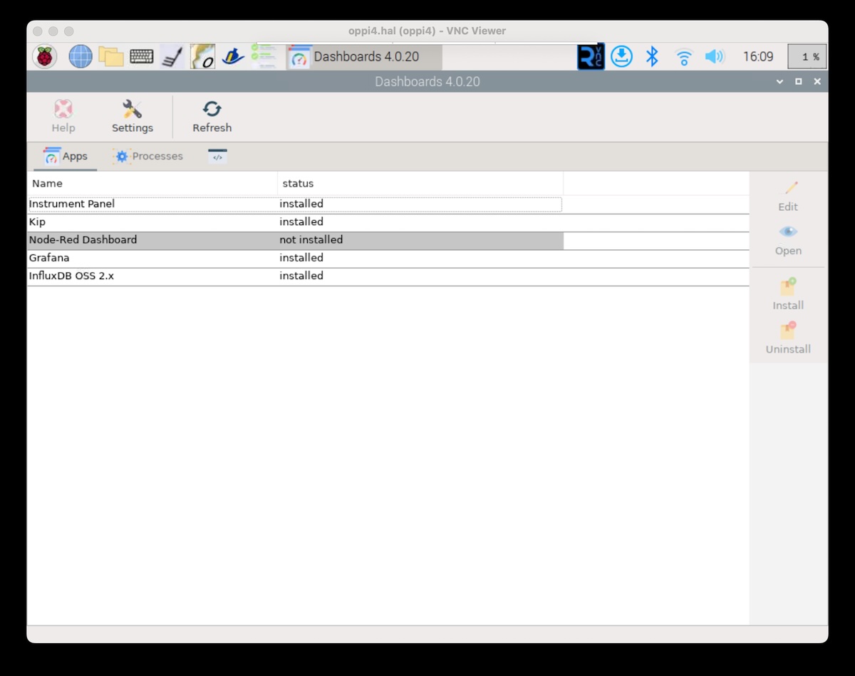
Install InfluxDB and Grafana.
Configure InfluxDB
Open InfluxDB with a browser (doesn’t have to be on the VNC): http://openplotter.local:8086/
- Click Get Started
- Create a user and fill in the following information:
- Username: admin
- Password: (select one)
- org: signalk
- initial bucket: signalk
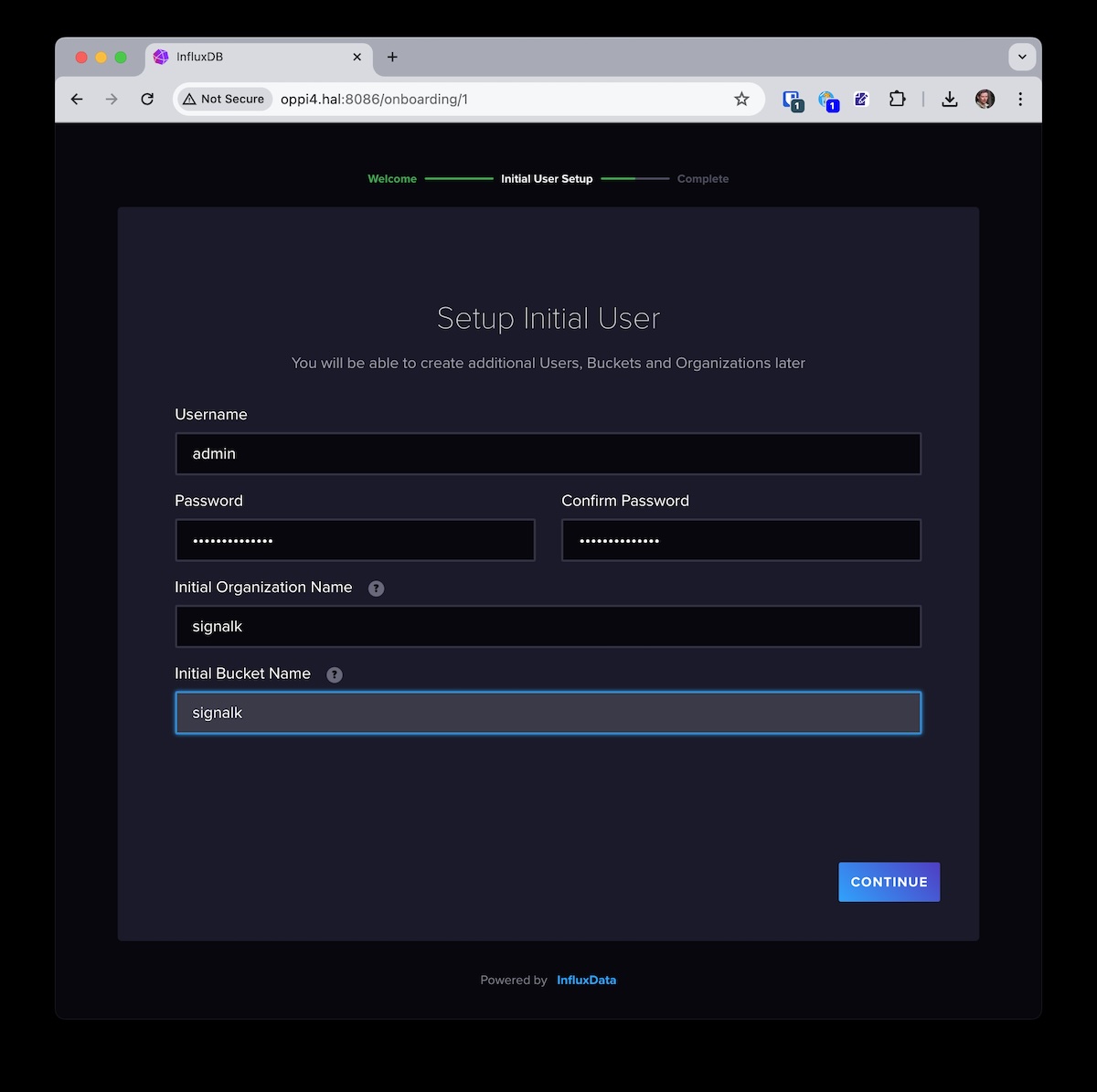
Setup the initial user as shown in the image.
Click Continue, and then copy the generated operator API token. You will need this later.
Configure the Signal K InfluxDB plugin
Now that we have InfluxDB set up and running, we want to configure Signal K to send data there.
- Go to Signal K web UI: http://openplotter.local:3000/ (Create an admin user if this is your first time here.)
Add the “Signal K to InfluxDb 2” plugin:
- Go to Appstore.
- Search for “influx”.
- Click Install on “Signal K to InfluxDb 2”.
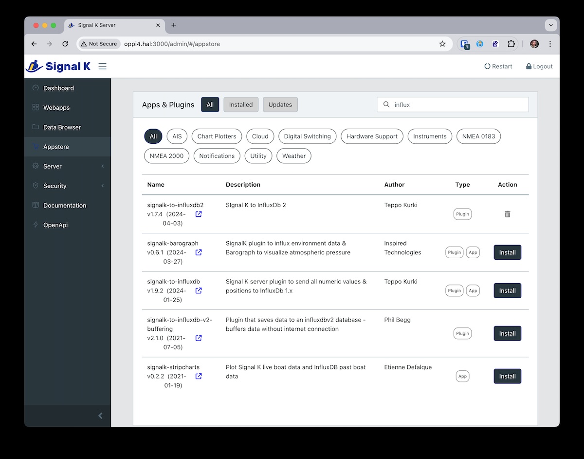
Install the signalk-to-influxdb2 plugin.
Restart Signal K to apply the changes.
Next, configure the plugin:
- Go to Server -> Plugin Config.
- Scroll down to “Signal K to InfluxDb 2”. Expand it.
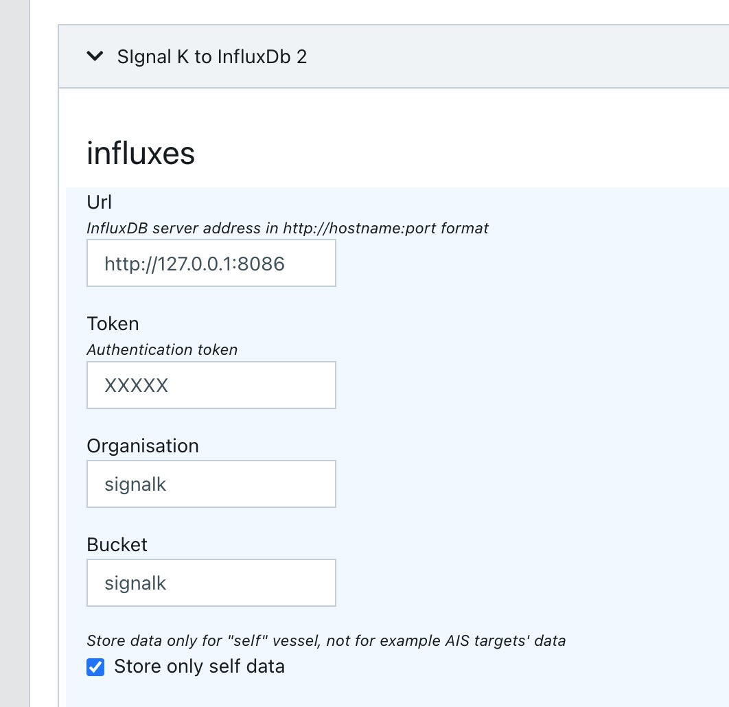
The plugin can connect to multiple InfluxDB instances. We will only use one:
- Add a new Influx instance
- Url: http://127.0.0.1:8086
- Set the token to the one you copied earlier
- Organization: signalk
- Bucket: signalk
If you’re mostly interested in your own boat data, select “Store only self data”. Leaving that unchecked may result in a lot of data being stored, especially if you are in a busy area.
Configure the InfluxDB plugin.
You can skip the ignored path and sources at this point. Come back later to play with the settings once you have some data.
Select “Use timestamps from SK data.” We want to store the data time as it was generated, not when it was saved to InfluxDB (even though the difference is usually insignificant – but we need to have some principles!).
“Resolution” is an important setting. It defines how often data is stored. Fastest NMEA 2000 updates happen every 100 ms, but that results in a lot of data. Usually something like 1000 ms or even slower is enough.
If you intend to view Grafana graphs in real-time, set “Flush interval” to 1000 ms. Otherwise, you can set it to a higher value like 5000 ms or 10 000 ms to improve disk write efficiency.
The remaining settings get pretty technical and can be safely skipped. Be sure to click “Submit” to save your settings!
At this point, Signal K should start sending data to InfluxDB. How exciting!
Configure Grafana
To view the data, we need to connect Grafana to InfluxDB and create a dashboard.
Login to Grafana: http://openplotter.local:3001/
At the first login, you might have to create a new admin user. When you’re in, you can create a new data source to make Grafana access the InfluxDB data:
- Click on “Add your first data source”
- Data source type: Influxdb
- Name: influxdb
- Query language: InfluxQL
- HTTP URL: http://localhost:8086
To authenticate, you need to add a custom HTTP header:
- Header: Authorization
- Value: Token (token from above)
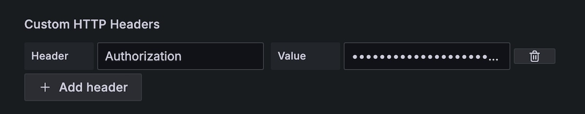
Add the Authorization header.
Use the following settings:
- Database: signalk
- HTTP Method: GET
- Min time interval: 1s
Then click “Save & test”. After a short while, you should get a positive acknowledgment.
Create a Dashboard
Dashboards are collections of graphs and other visualizations. That’s where you can see your data in a more human-friendly way. We’ll just create a simple graph for now:
- Go back to Grafana Home menu
- Hamburger menu -> Dashboards -> Create Dashboard
- Add visualization
- Data source: influxdb
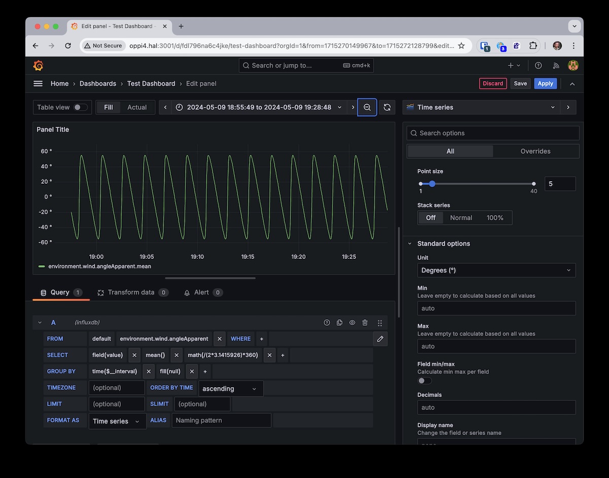
Panel editing view.
Wait, what?
Before we continue, let’s have a quick explanation of how the data is stored. Under the surface, Signal K (and mostly NMEA 2000 as well) stores all of its data in SI units. That means that the boat speed is stored in m/s, wind angle in radians, and so on.
This may sound weird because everyone knows that boat speed is in knots, wind angle in degrees, water depth in fathoms and anchor weight in stones. However, always sticking to SI units makes the stored data unambiguous. If we know the measurement type (e.g. temperature), we know the unit (Kelvin). It is then the responsibility of the display layer (a dashboard, plotter app, Grafana graph) to convert the data to the desired units.
(This approach is not designed to annoy just those using imperial units. Using Kelvins and radians is equally annoying to everyone. But it is still the right way. Trust us. Principles, you know.)
In the “A” query, click “select measurement” and select a measurement (e.g. environment.wind.angleApparent)
The value is in radians. Let’s convert it to degrees. Click the plus sign on the SELECT row. Select “math”.
Edit the math expression: / (2 * 3.14159265) * 360. This converts radians to degrees.
In the right hand side column, scroll down to “Standard options”. Select Unit and pick Degrees. This tells Grafana that the data, after conversion, is in degrees.
You should now have a minimal graph showing wind angle in degrees! Congratulations!
4 - Tutorials and Example Projects
HALPI tutorials and example projects will be listed on this page.
5 - Errata
This page lists all known hardware bugs for different HALPI revisions.